
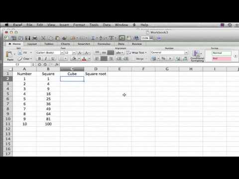
Q. How do you write an exponent formula in Excel?
How to Type Exponents in Excel
- Click on the cell where you want to type the exponent.
- Type the “=” sign. This sign informs Excel that you are entering a formula.
- Type the base number. For example, type “3.”
- Type the “^” symbol, located on the 6 key on a standard keyboard.
- Type the exponent.
- Press the “Enter” key.
Q. What is power formula in Excel?
The Excel POWER function returns a number to a given power. The POWER function works like an exponent in a standard math equation. Raise a number to a power. Number raised to power. =POWER (number, power)
Q. How do you write a power formula?
Enter a caret — “^” — into the formula bar, then enter the power. For example, to multiply 3 to the power of 4, enter “3^4” and press “Enter” to complete the formula.
Q. How do you do standard form on Excel?
When cells are in General format, you can type scientific notation directly. Enter the number, plus “E,” plus the exponent. If the number is less than zero, add a minus sign before the exponent. Note that Excel will automatically use Scientific format for very large and small numbers of 12 or more digits.
Q. How do you automatically fill serial number in Excel without dragging?
Quickly Fill Numbers in Cells without Dragging
- Enter 1 in cell A1.
- Go to Home –> Editing –> Fill –> Series.
- In the Series dialogue box, make the following selections: Series in: Columns. Type: Linear. Step Value: 1. Stop Value: 1000.
- Click OK.
Q. Where is the fill handle in Excel?
The fill handle will appear as a small square in the bottom-right corner of the selected cell(s). Click, hold, and drag the fill handle until all of the cells you want to fill are selected.
Q. Why is fill down not working in Excel?
If you’re still having an issue with drag-to-fill, make sure your advanced options (File –> Options –> Advanced) have “Enable fill handle…” checked. You might also run into drag-to-fill issues if you’re filtering. Try removing all filters and dragging again.
Q. What is an absolute cell reference in Excel?
In contrast, the definition of absolute cell reference is one that does not change when it’s moved, copied or filled. This way, the reference points back to the same cell, no matter where it appears in the workbook. It’s indicated by a dollar sign in the column or row coordinate.
Q. How do you create an absolute cell reference in Excel?
Create an Absolute Reference
- Click a cell where you want to enter a formula.
- Type = (an equal sign) to begin the formula.
- Select a cell, and then type an arithmetic operator (+, -, *, or /).
- Select another cell, and then press the F4 key to make that cell reference absolute.
Q. How do you use an absolute cell reference in Excel without F4?
If you’re running MAC, use the shortcut: ⌘ + T to toggle absolute and relative references. You can’t select a cell and press F4 and have it change all references to absolute.
Q. What is mixed cell reference in Excel?
Mixed reference in excel is a type of cell reference which is different from the other two absolute and relative, in mixed cell reference we only refer to the column of the cell or the row of the cell, for example in cell A1 if we want to refer to only A column the mixed reference would be $A1, to do this we need to …
Q. How do you do a relative cell reference in Excel?
To create and copy a formula using relative references:
- Select the cell that will contain the formula.
- Enter the formula to calculate the desired value.
- Press Enter on your keyboard.
- Locate the fill handle in the bottom-right corner of the desired cell.
- Click and drag the fill handle over the cells you want to fill.
Q. How do you use a relative cell reference formula?
Use cell references in a formula
- Click the cell in which you want to enter the formula.
- In the formula bar. , type = (equal sign).
- Do one of the following, select the cell that contains the value you want or type its cell reference.
- Press Enter.
Q. What is a structured reference formula in Excel?
A structured reference is a term for using a table name in a formula instead of a normal cell reference. Structured references are optional, and can be used with formulas both inside or outside an Excel table.
Q. How do you create a structured reference formula?
To include structured references in your formula, click the table cells you want to reference instead of typing their cell reference in the formula. Let’s use the following example data to enter a formula that automatically uses structured references to calculate the amount of a sales commission.
Q. How do you create a structured reference formula in Excel?
Structured References
- Select cell E1, type Bonus, and press Enter.
- Select cell E2 and type =0.02*[
- Close with a square bracket and press Enter.
- Note: click AutoCorrect Options and click Undo Calculated Column to only insert the formula into cell E2.
- Select cell E18 and enter the formula shown below.
Q. Why we use Sumif formula in Excel?
SUMIF is the function used to sum the values according to a single criterion. Using this function, you can find the sum of numbers applying a condition within a range. This function comes under Math & Trigonometry functions. Similar to the name, this will sum if the criteria given is satisfied.
Q. Why is my Sumif not working?
If you are writing the correct formula and when you update sheet, the SUMIF function doesn’t return updated value. It is possible that you have set formula calculation to manual. Press F9 key to recalculate the sheet. Check the format of the values involved in the calculation.
Q. How do I fix Sumif?
Solution: Open the workbook indicated in the formula, and press F9 to refresh the formula. You can also work around this issue by using SUM and IF functions together in an array formula. See the SUMIF, COUNTIF and COUNTBLANK functions return #VALUE!
Q. Why is my Sumif returning wrong value?
The issue is that your criteria range (B3) and sum range (C3:I3) are not the same size, so your sum range is trimmed to match the size of the criteria range, effectively only summing C3. It works the same way if the sum range is larger than the criteria range.
Q. How do you do a sum if error in Excel?
Sum Range with Errors
- We use the IFERROR function to check for an error. Explanation: the IFERROR function returns 0, if an error is found.
- To sum the range with errors (don’t be overwhelmed), we add the SUM function and replace A1 with A1:A7.
- Finish by pressing CTRL + SHIFT + ENTER.
Q. How do you get Excel to ignore a formula?
If the formula is not an error you can choose to ignore it:
- Click Formulas > Error Checking.
- Then click Ignore Error.
- Click OK or Next to jump to the next error.
How to Type Exponents in Excel
- Click on the cell where you want to type the exponent.
- Type the “=” sign. This sign informs Excel that you are entering a formula.
- Type the base number. For example, type “3.”
- Type the “^” symbol, located on the 6 key on a standard keyboard. Advertisement.
- Type the exponent. For example, type “2.”
- Press the “Enter” key.
Q. How do you show a power in Excel?
Keyboard shortcuts for superscript and subscript in Excel
- Select one or more characters you want to format.
- Press Ctrl + 1 to open the Format Cells dialog box.
- Then press either Alt + E to select the Superscript option or Alt + B to select Subscript.
- Hit the Enter key to apply the formatting and close the dialog.
An absolute reference in Excel refers to a reference that is “locked” so that rows and columns won’t change when copied. Unlike a relative reference, an absolute reference refers to an actual fixed location on a worksheet. To create an absolute reference in Excel, add a dollar sign before the row and column.
Q. How do you use Counta and Countif?
We can use a combination of the COUNTA, COUNTIF, and SUMPRODUCT functions to get the desired results. We can list down the things we wish to exclude from counting. One other way to arrive at the same result is to use the formula =COUNTIFS(B4:B9,”<>Rose”B4:B9,”<>Marigold”).
Q. What is the difference between Counta and Countblank?
Introducing COUNTA, COUNTBLANK and COUNTIF COUNT counts how many cells in a range contain numeric data (numbers). COUNTA counts how many populated cells in a range (i.e. not blank). COUNTBLANK counts how many blank cells in a range.
Q. What is the difference between Count and Dcount?
COUNT counts the number of items being aggregated. D_COUNT counts the number of unique items there are being aggregated.
Q. What is Dcount function?
The Excel DCOUNT function counts matching records in a database using criteria and an optional field. When a field is provided DCOUNT will only count numeric values in the field. Use DCOUNTA to count numbers or text values in a given field.
Q. What is Daverage in Excel?
The Excel DAVERAGE function returns the average in a given field for records that match criteria. Get average from matching records. The average value in a given field. =DAVERAGE (database, field, criteria) database – Database range including headers.
Q. What is access Dcount?
You can use the DCount function to count the number of records containing a particular field that isn’t in the record source on which your form or report is based. If you use an ampersand to separate the fields, the DCount function returns the number of records containing data in any of the listed fields.
Q. What is DSum access?
DSum() Function : In MS Access, the DSum() function is used to calculate the sum of a set of values in a specified set of records (a domain). The DSum functions return the sum of a set of values from a field that satisfy the criteria.
Q. How do I find the row number in an Access query?
Another way to assign a row number in a query is to use the DCount function. It doesn’t rely on the order of the table, either – the RowID is calculated on its actual value and those that are less than it. This method can be applied to any (primary key) type (e.g. Number , String or Date ).